Problems tagged with "linear prediction functions"
Problem #002
Tags: linear prediction functions
Suppose a linear prediction rule \(H(\vec x; \vec w) = \Aug(\vec x) \cdot\vec w\) is parameterized by the weight vector \(\vec w = (3, -2, 5, 2)^T\). Let \(\vec z = (1, -1, -2)^T\). What is \(H(\vec z)\)?
Solution
-8
Problem #004
Tags: linear prediction functions
Suppose a linear predictor \(H_1\) is fit on a data set \(X = \{\nvec{x}{i}, y_i\}\) of \(n\) points by minimizing the mean squared error, where each \(\nvec{x}{i}\in\mathbb R^d\).
Let \(Z = \{\nvec{z}{i}, y_i\}\) be the data set obtained from the original by standardizing each feature. That is, if a matrix were created with the \(i\)th row being \(\nvec{z}{i}\), then the mean of each column would be zero, and the variance would be one.
Suppose a linear predictor \(H_2\) is fit on this standardized data by minimizing the mean squared error.
True or False: \(H_1(\nvec{x}{i}) = H_2(\nvec{z}{i})\) for each \(i = 1, \ldots, n\).
Solution
True.
Problem #006
Tags: linear prediction functions
Let \(\nvec{x}{1} = (-1, -1)^T\), \(\nvec{x}{2} = (1, 1)^T\), and \(\nvec{x}{3} = (-1, 1)^T\). Suppose \(H\) is a linear prediction function, and that \(H(\nvec{x}{1}) = 2\) while \(H(\nvec{x}{2}) = -2\) and \(H(\nvec{x}{3}) = 0\).
Let \(\nvec{x}{4} = (1,-1)^T\). What is \(H(\nvec{x}{4})\)?
Solution
0
Problem #019
Tags: linear prediction functions
Suppose a linear prediction rule \(H(\vec x; \vec w) = \Aug(\vec x) \cdot\vec w\) is parameterized by the weight vector \(\vec w = (2, 1, -3, 4)^T\). Let \(\vec z = (3, -2, 1)^T\). What is \(H(\vec z)\)?
Solution
15
Problem #023
Tags: linear prediction functions
Let \(\nvec{x}{1} = (-1, -1)^T\), \(\nvec{x}{2} = (1, 1)^T\), and \(\nvec{x}{3} = (-1,1)^T\). Suppose \(H\) is a linear prediction function, and that \(H(\nvec{x}{1}) = 2\), \(H(\nvec{x}{2}) = -2\), and \(H(\nvec{x}{3}) = 2\).
Let \(\vec z = (2,-1)^T\). What is \(H(\vec z)\)?
Solution
-4
Problem #060
Tags: linear prediction functions
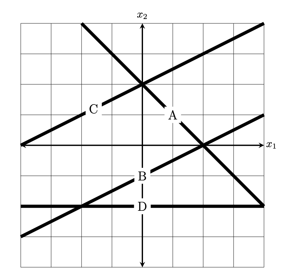
Suppose a linear prediction function \(H(\vec x) = w_0 + w_1 x_1 + w_2 x_2\) is trained to perform classification, and the weight vector is found to be \(\vec w = (2, -1, 2)^T\).
The figure below shows four possible decision boundaries: \(A\), \(B\), \(C\), and \(D\). Which of them is the decision boundary of the prediction function \(H\)?
You may assume that each grid square is 1 unit on each side, and the axes are drawn to show you where the origin is.

Solution
B.
Here are four ways to solve this problem:
Method 1: Guess and check, using the fact that $H(\vec x)$ must equal zero at every point along the decision boundary. For any of the proposed decision boundaries, we can take a point on the boundary, compute \(H(\vec x)\), and see if it equals 0.
Consider option \(A\), and take an arbitrary point on that boundar -- for example, the point \((1, 1)^T\). Computing \(H(\vec x)\), we get \(H(\vec x) = \vec w \cdot\operatorname{Aug}(\vec x) = (2, -1, 2) \cdot(1, 1, 1) = 3 \neq 0\). Therefore, this cannot be the decision boundary.
Considering option \(B\), it looks like the point \((0, -1)^T\) is on the boundary, Computing the value of \(H\) here, we get \(H(\vec x) = \vec w \cdot\operatorname{Aug}(\vec x) = (2, -1, 2) \cdot(1, -1, 1) = 0\). That's a good sign, but it's not sufficient to say that this must be the decision boundary (at this point, all we can say is that whatever the decision boundary is, it must go through \((0, -1)\).) To make sure, we pick a second point on the boundary, say, \((2, 0)^T\). Computing \(H\) at this point, we get \(H(\vec x) = \vec w \cdot\operatorname{Aug}(\vec x) = (2, -1, 2) \cdot(1, 2, 0) = 0\). With this, we can conclude that \(B\) must be the decision boundary.
Method 2: Use the fact that $(w_1, w_2)$ is orthogonal to the decision boundary. In Homework 02, we learned a useful way of relating the decision boundary to the weight vector \(\vec w = (w_0, w_1, w_2)^T\): it is orthogonal to the vector \(\vec w' = (w_1, w_2)^T\).
In this case, \(\vec w' = (-1, 2)^T\); this is a vector that up and to the left (more up than left). This rules out options \(A\) and \(D\), since they can't be orthogonal to that vector. There are several ways to decide between \(B\) and \(C\), including the logic from Method 1.
Method 3: Find the equation of the decision boundary in $y = mx + b$ form. Another way to solve this problem is to find the equation of the decision boundary in familiar ``\(y = mx + b\)'' form. We can do this by setting \(H(\vec x) = 0\) and solving for \(x_2\) in terms of \(x_1\). We get:
Plugging in \(w_0 = 2\), \(w_1 = -1\), and \(w_2 = 2\), we get
So the decision boundary is a line with slope \(-\frac{1}{2}\) and \(y\)-intercept \(-1\). This is exactly the equation of the line in option \(B\).
Method 4: reasoning about the slope in each coordinate. Similar to Method 2, we can rule out options \(A\) and \(D\) by reasoning about the slope of the decision boundary in each coordinate.
Imagine this scenario: you're standing on the surface of \(H\) at a point where \(H = 0\)(that is, you're on the decision boundary). You will take one step to the right (i.e., one step in the \(x_1\) direction), which will (in general) cause you to leave the decision boundary and either increase or decrease in height. If you want to get back to the decision boundary, and your next step must be either up or down, which should it be? The answer will tell you whether the decision boundary looks like \(/\) or like \(\backslash\).
In this case, taking a step to the right (in the \(x_1\) direction) will cause you to decrease in height. This is because the \(w_1\) component of \(\vec w\) is negative, and so increasing \(x_1\) will decrease \(H\). Now, to get back to the decision boundary, you must increase your height to get back to \(H = 0\). Since the slope in the \(x_2\) direction is positive (2, to be exact), you must increase\(x_2\) in order to increase \(H\). Therefore, the decision boundary is up and to the right: it looks like \(/\).
Problem #061
Tags: feature maps, linear prediction functions
Suppose a linear prediction function \(H(\vec x) = w_1 \phi_1(\vec x) + w_2 \phi_2(\vec x) + w_3 \phi_3(\vec x) + w_4 \phi_4(\vec x)\) is fit using the basis functions
where \(\vec x = (x_1, x_2)^T\) is a feature vector in \(\mathbb R^2\). The weight vector \(\vec w\) is found to be \(\vec w = (1, -2, 3, -4)^T\).
Let \(\vec x = (1, 2)^T\). What is \(H(\vec x)\)?
Solution
We have:
Problem #063
Tags: linear prediction functions
Suppose a linear prediction function \(H(\vec x) = w_0 + w_1 x_1 + w_2 x_2\) is fit to data and the following are observed:
At a point, \(\nvec{x}{1} = (1, 1)^T\), the value of \(H\) is 4.
At a point, \(\nvec{x}{2} = (1, 0)^T\), the value of \(H\) is 0.
At a point, \(\nvec{x}{3} = (0, 0)^T\), the value of \(H\) is -4.
What is the value of \(H\) at the point \(\nvec{x}{4} = (0, 1)^T\)?
Solution
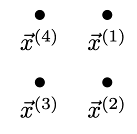
The four points make a square:

Since \(H = 0\) at \(\nvec{x}{2}\), the decision boundary must pass through that point. And since \(H(\nvec{x}{1}) = 4 = -H(\nvec{x}{3})\), the points \(\nvec{x}{1}\) and \(\nvec{x}{3}\) are equidistant from the decision boundary. Therefore, the decision boundary must pass exactly halfway between \(\nvec{x}{1}\) and \(\nvec{x}{3}\). This makes a line going through \(\nvec{x}{4}\), meaning that \(\nvec{x}{4}\) is on the decision boundary, so \(H(\nvec{x}{4}) = 0\).
Problem #078
Tags: linear prediction functions
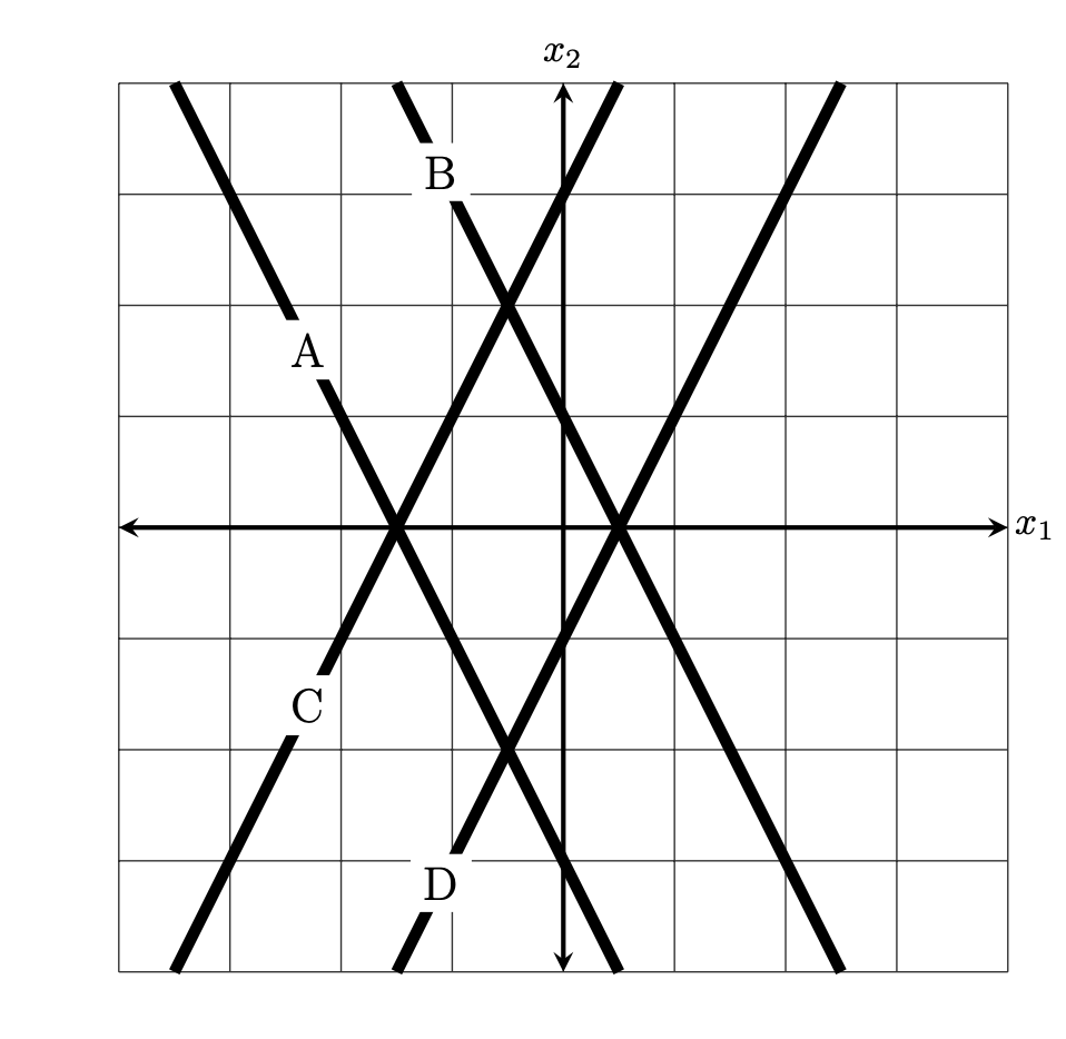
Suppose a linear prediction function \(H(\vec x) = w_0 + w_1 x_1 + w_2 x_2\) is trained to perform classification, and the weight vector is found to be \(\vec w = (1,-2,1)^T\).
The figure below shows four possible decision boundaries: \(A\), \(B\), \(C\), and \(D\). Which of them is the decision boundary of the prediction function \(H\)?
You may assume that each grid square is 1 unit on each side, and the axes are drawn to show you where the origin is.

Solution
D.
Problem #079
Tags: feature maps, linear prediction functions
Suppose a linear prediction function \(H(\vec x) = w_1 \phi_1(\vec x) + w_2 \phi_2(\vec x) + w_3 \phi_3(\vec x) + w_4 \phi_4(\vec x)\) is fit using the basis functions
where \(\vec x = (x_1, x_2, x_3)^T\) is a feature vector in \(\mathbb R^3\). The weight vector \(\vec w\) is found to be \(\vec w = (2, 1, -2, -3)^T\).
Let \(\vec x = (1, 2, 1)^T\). What is \(H(\vec x)\)?
Problem #080
Tags: least squares, linear prediction functions
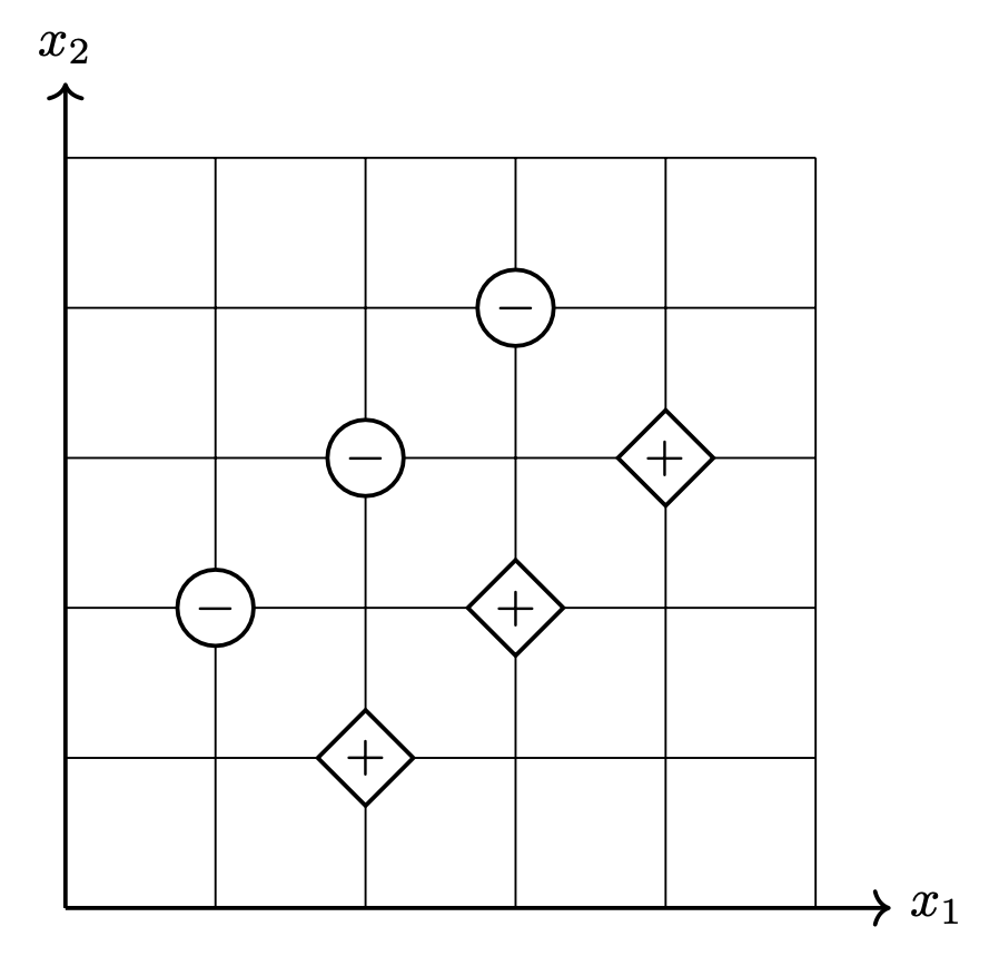
Consider the binary classification data set shown below consisting of six points in \(\mathbb R^2\). Each point has an associated label of either +1 or -1.

What is the mean squared error of a least squares classifier trained on this data set (without regularization)? Your answer should be a number.